
- boostcourse
- 기초다지기
- 이기적
- 빅분기
- 파이썬
- AI 플랫폼을 활용한 데이터 분석
- 빅데이터 분석 기반 에너지 운영 관리자 양성 및 취업과정
- boostcoures
- 정보처리기사
- r
- 데이터 분석 기반 에너지 운영 관리자 양성 및 취업과정
- 난생처음 R코딩&데이터 분석 저서
- 데이터베이스
- PY4E
- 빅데이터분석기사
- DB
- Machine Learning
- 코딩테스트 python
- [멀티잇]데이터 시각화&분석 취업캠프(Python)
- Ai
- python
- 코딩테스트
- 프로그래머스
- 부스트코스
- 네이버부스트캠프
- Oracle
- 이것이 취업을 위한 코딩테스트다 with 파이썬
- SQL
- 오라클
- 인공지능기초다지기
- Today
- Total
매일공부
[Machine Learning] 로지스틱 회귀분석(분류) 본문
Logistic Regression
- S자로 선을 그어서 데이터가 특정 카테고리에 속할지를 0과 1사이의 연속적인 확률로 예측하는 회귀 알고리즘
- 종속변수 : 범주형 데이터
- 입력 데이터가 주어졌을 때 결과가 특정 분류로 나누기 위한 분류 기법

Logistic Regression 가정
- 응답변수가 범주형 데이터값(이진)
- 독립변수는 본질적으로 서로 독립적(다중 공선성이 거의 또는 전혀 없어야 함)
- log-odds와 독립 변수는 선형적으로 연관되어야 함
- 로지스틱 회귀는 대규모 크기 샘플에만 적용해야 합니다.
종류
- 이진 로지스틱 회귀 : 범주형 응답에 대해 가능한 결과는 두 가지 예) 합격하거나 불합격
- 다항 로지스틱 회귀: 범주형 응답변수에 순서가 없는(X) 3개 이상의 변수가 포함된 경우 로지스틱 회귀 분석 모델
- 순서 로지스틱 회귀: 범주형 응답변수에 순서가 있는(O) 3개 이상의 변수가 포함된 경우 로지스틱 회귀 분석 모델
Odds (승산)
- P(A) / 1-P(A) = 임의의 사건 A 발생할 확률 / 발생하지 않을 확률
- 범위 = 0 ~ 양의 무한대의 값
Log-odds (로그 오즈)
- positive class에 속할 확룔
- odds에 log를 취한 것
- 0과 양의 무한대의 값을 범위로 가지는 Odds를 음의 무한대부터 양의 무한대까지의 범위를 갖도록 하는 방법
Sigmoid Function (시그모이드 함수)
- log-odds인 z 값을 취해서 0 과 1 사이의 값을 반환
- 공식 : 1/(1+e^-z) z = log-odds
- Logistic Regression이 특정 데이터가 positive class에 속할 확률을 계산

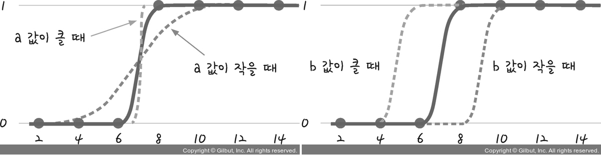
| a값 | b값 | |
| 작아질수록(↓) | 오차 무한대 ∞ | 오차 무한대 ∞ |
| 커질수록(↑) | 오차 무한대로 커짐X |
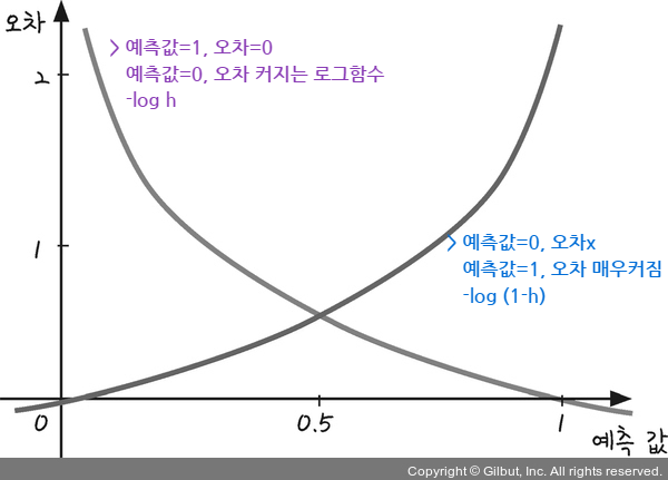
오차계산
- 로지스틱 회귀분석에서는 평균제곱 오차로 오차 계산X => 교차 엔트로피 함수 사용
- a, b 값 > 경사하강법 사용
- y = [0,1]
로지스틱 회귀로 분류를 수행한다는 의미
- 회귀 분석 결과인 연속변수 예측값을 시그모이드 함수로 표준화시켜서 임계값 기준으로 나누어서 분류를 수행함
- y = w1x1 + w2x2 + ..... + wnxn + b
- 가중치 w1, w2, w3, w4, w5와 b(bias 편향) : 비용함수를 통해 최적의 값을 훈련과정을 통해 구함
단점
= 선형방식의 회귀분석 모델이므로 고급 분석 모델에 비해 비선형에 취약
#다항 로지스틱회귀
- 이진 클래스 분류
: 양성 클래스에 대한 log_odds(z)값만 계산
=> 하나의 z값만으로 다른 클래스의 확률을 유추(시그모이드 함수) - 다중 클래스 분류
: 각 클래스마다 log_odds(z)값 계산
=> softmax함수로 z값을 확률로 변환

Softmax Function (소프트맥스 함수)
- 예측 값을 0~1 사이의 값으로 주여주고 모든 입력값의 합이 1이 되도록 줄여줌
- 각 클래스의 z값을 지수로 하는 자연상수 e를 모두 더한값을 분모로 하고, 각각의 z값을 지수로 하는 자연상수 e를 분자로 나누면 해당클래스의 z값의 확률로 계산됨
C 파라미터 : 규제
(LinearRegression의 규제파라미터 지만, C는 값이 작을수록 규제 정도가 세진다)
#Logistic Regression 하이퍼파라미터
- LogisticRegression( C= , max_iter=)
- max_iter : 훈련 반복 횟수 (최소값 100)
- solver: {‘newton-cg’, ‘lbfgs’, ‘liblinear’, ‘sag’, ‘saga’}, default=’lbfgs’ #최적화 문제에 사용할 알고리즘
- penalty: {‘l1’, ‘l2’, ‘elasticnet’, ‘none’}, default=’l2
- C: float, default=1.0 #규제 : 작을수록 규제 정도 세짐 (alpha는 값이 커지면 규제 정도가 세짐)
예시코드]
from sklearn.linear_model import LogisticRegression
hyperparameters = {
    'solver'  : ['newton-cg', 'lbfgs', 'liblinear'],
    'penalty' : ['l2'],
    'C'       : [100, 10, 1.0, 0.1, 0.01]
}
# 실습
# 피마 인디언의 당뇨병 데이터 셋 - 텐서플로우 로지스틱 회귀분석
- Pregnancies: 임신 횟수
- Glucose: 포도당 부하 검사 수치
- BloodPressure: 혈압(mm Hg)
- SkinThickness: 팔 삼두근 뒤쪽의 피하지방 측정값(mm)
- Insulin: 혈청 인슐린(mu U/ml)
- BMI: 체질량지수(체중(kg)/(키(m))^2)
- DiabetesPedigreeFunction: 당뇨 내력 가중치 값
- Age: 나이
- Outcome: 클래스 결정 값(0또는 1)
diabetes_data = pd.read_csv('./datas/diabetes.csv')
print(diabetes_data['Outcome'].value_counts())
diabetes_data.info()

X=diabetes_data.iloc[:, :-1]
y=diabetes_data.iloc[:, -1]

#학습 , 테스트 데이터 셋 분할 (test_size=0.25,random_state=1)
X_train, X_test, y_train, y_test = train_test_split(X, y, test_size=0.25, random_state=1

from sklearn.linear_model import LogisticRegression
logreg = LogisticRegression(random_state=1)
logreg.fit(X_train, y_train)
y_pred = logreg.predict(X_test)

from sklear. metrics import confusion_matrix
cnf_matrix = confusion_matrix(y_test, y_pred)
print(cnf_matrix )

class_names=[0,1]
fig, ax = plt.subplots()
tick_marks = np.arange(len(class_names))
plt.xticks(tick_marks, class_names)
plt.yticks(tick_marks, class_names)
sns.heatmap(pd.DataFrame(cnf_matrix), annot=True, cmap="YlGnBu" ,fmt='g')
ax.xaxis.set_label_position("top")
plt.tight_layout()
plt.title('Confusion matrix', y=1.1)
lt.ylabel('Actual label')
plt.xlabel('Predicted label')
Text(0.5,257.44,'Predicted label');

from sklearn.metrics import classification_report
target_names = ['without diabetes', 'with diabetes']
print(classification_report(y_test, y_pred, target_names=target_names))

#ROC : 거짓 양성 비율에 대한 실제 양성 비율 그래프 (민감도 , 특이도 사이의 균형)
from sklearn.metrics import roc_curve, roc_auc_score
y_pred_proba = logreg.predict_proba(X_test)[::,1]
fpr, tpr, _ = roc_curve(y_test,  y_pred_proba)
auc = roc_auc_score(y_test, y_pred_proba)
plt.plot(fpr,tpr,label="data 1, auc="+str(auc))
plt.legend(loc=4)
plt.show()
# 다항 로지스틱회귀
import pandas as pd
fish = pd.read_csv('./datas/fish.csv')
fish.info()

# 예측할 품종의 종류(label) 확인
print(pd.unique(fish['Species'])

#데이터의 feature(특성)과 label(정답)을 분리
fish_input = fish.iloc[:, 1:].to_numpy()
fish_target = fish.iloc[:,1].to_numpy()
print(fish_input[:5])
print(fish_target[:5])

fish_input.describe()

#학습, 테스트 데이터셋 분할
X_train, X_test, Y_train, Y_test = train_test_split(fish_input, fish_target, test_size=0.25, random_state=42)

#feature 데이터 정규화
from sklearn.preprocessing import StandardScaler
ss=StandardScaler()
train_scaled =ss.fit_transform(X_train)
test_scaled =ss.fit_transform(X_test)
print(pd.DataFrame(train_scaled).describe())

#Y(Species) = w1*(Weight) + w2*(Length) + w3*(Diagonal) + w4*(Height) + w5*(Width) + b

lr=LogisticRegression(C=20,max_iter=1000)
lr.fit(train_scaled, Y_train)

print(lr.score(train_scaled, Y_train))  #성능 평가
print(lr.score(test_scaled, Y_test))
print(lr.predict(test_scaled[:5]) )  #테스트 데이터 상위 5개만 예측
proba = lr.predict_proba(test_scaled[:5])   ##테스트 데이터 상위 5개 예측 확률
print(lr.classes_)    #모델의 예측 클래스 종류
print(np.round(proba, decimals=3))

#회귀계수와 bias 확인
print(lr.coef_.shape)
print(lr.intercept_.shape)
#클래스가 7개이므로 클래스별 분류에 적용되는 회귀계수와 bias값이 모두 다름
for i in range(7):
    print(lr.coef_[i], lr.intercept_[i])

#분류 클래스별 확률 기반으로 Y값을 출력해주는 함수
decision = lr.decision_function(test_scaled[:5])
print(np.round(decision, decimals=2))
# 인공신경망 라이브러리 tensorflow와 keras 기반 다중 클래스 분류 실습
df = pd.read_csv('./datas/iris.csv')
df.info()
df.head()

import seaborn as sns
import matplotlib.pyplot as plt

sns.pairplot(df, hue='species') #hue 옵션은 주어진 데이터 중 어떤 카테고리를 중심으로 시각화할지 설정
plt.show()

X =df.iloc[:, :4]
y = df.iloc[:, 4]

print(X[:5])
print(y[:5])

y =pd.get_dummies(y)
print(y[:5])


##은닉층은 몇 층으로 할지, 은닉층 안의 노드는 몇 개로 할지에 대한 정답은 없습니다.
## 노드의 수와 은닉층의 개수를 바꾸어 보면서 더 좋은 정확도가 나오는지 확인해보세요
import tensorflow as tf
from tensorflow.keras.models import Sequential
from tensorflow.keras.layers import Dense

model = Sequential()
model.add(Dense(12, input_dim=4, activation='relu'))
model.add(Dense(8, activation='relu'))
model.add(Dense(3, activation='softmax'))
model.summary()

model.compile(loss='categorical_crossentropy', optimizer='adam', metrics=['accuracy'])

history = model.fit(X, y, epochs=100, batch_size=10)
'IT > ML' 카테고리의 다른 글
| [sklearn] 의사결정트리(Decision Tree) (0) | 2022.11.03 |
|---|---|
| [Machine Learning] TensorFlow, Keras (0) | 2022.11.03 |
| [sklearn] 모델 정확도 평가; 오차측정 지표 (0) | 2022.11.03 |
| Machine Learning 수업 전체 흐름 & 키워드 (0) | 2022.11.03 |
| [Machine Learning] 인공지능이란? (0) | 2022.11.03 |


