
- 네이버부스트캠프
- 빅데이터 분석 기반 에너지 운영 관리자 양성 및 취업과정
- Machine Learning
- 파이썬
- 빅분기
- 코딩테스트
- PY4E
- Ai
- 이기적
- boostcoures
- SQL
- 오라클
- 난생처음 R코딩&데이터 분석 저서
- 데이터베이스
- 데이터 분석 기반 에너지 운영 관리자 양성 및 취업과정
- Oracle
- 빅데이터분석기사
- DB
- [멀티잇]데이터 시각화&분석 취업캠프(Python)
- 코딩테스트 python
- 부스트코스
- 프로그래머스
- r
- 이것이 취업을 위한 코딩테스트다 with 파이썬
- 정보처리기사
- 인공지능기초다지기
- boostcourse
- python
- AI 플랫폼을 활용한 데이터 분석
- 기초다지기
- Today
- Total
매일공부
[Machine Learning] 비계층적 군집분석; K-means, DBSCAN 본문
계층적 군집분석 : https://dailystudy.tistory.com/104
비계층적(확인적) 군집분석
1. K-mean clustering
- 거리 기반 알고리즘
- 평균 좌표를 이용해서 중심점을 반복적으로 업데이트하며 k개의 군집 형성
- 각 그룹 거의 동일한 분산 (크기 균형)
- 모든 특성은 동일한 스케일 가정(표준화 필수)
- 계층적 군집분석보다 속도 빠름
- 군집의 수를 알고 있는 경우 이용
- 변수보다 관측대상 군집화에 많이 이용
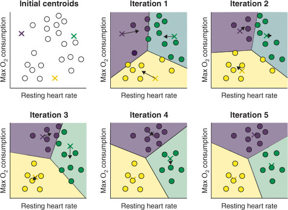
학습과정
- k개의 클러스터 '중심' 포인트를 랜덤한 위치에 생성
- 각 샘플에 대해
- 샘플과 k개의 중심 포인트 사이 거리 계산
- 샘플을 가장 가까운 중심 포인트의 클러스터에 할당
- 중심 포인트를 해당하는 클러스터의 평균(중심)으로 이동
- 더 이상 샘플의 클러스터 소속이 바뀌지 않을 때까지 단계 2, 3 반복
최적의 k값 설정
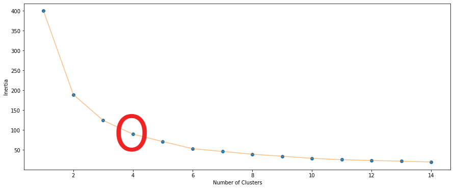
1. Elbow method
- inertia값 시각화 했을 때, 클러스터 수가 늘어감에 따라 inertia가 급격하게 감소하다가 완만하게 감소하면서 꺾이는 지점(Elbow) = 최적의 k(클러스터) 값
- WSS를 통해 비율의 한계비용(marginal cost)이 완곡하게 줄어드는 지점 = 최적의 k(클러스터) 값
- Inertia
: 군집의 응집도
: 군집 내 각 샘플과 가장 가까운 centroid 사이의 평균 제곱 거리 - 비율 고려 = 군집 간 분산(BSS) / 전체 분산(TSS) = (TSS - WSS) / TSS
> TSS = BSS + WSS
> WSS(Within cluster Sum of Squares) : 각 군집의 중심(centroid)와 각 군집에 속한 개체간 거리의 제곱합 - Inertia vs 클러스터 개수(군집개수) = 반비례 관계
- intertia가 낮을 수록 좋은 모델
2. Silhouette method
- 객체와 그 객체가 속한 군집의 데이터들과의 비유사성(dissimilarity)을 계산하는 방법
- (클러스터들간의 평균 거리 최소값 - 동일한 클러스터내 데이터들의 평균거리)
_____________________________________________________________
max(클러스터들간의 평균 거리 최소값, 동일한 클러스터내 데이터들의 평균거리) - 범위 (-1) ~ (+1)
> +1에 가까운 경우 : 해당 샘플이 cluster 안에 잘 속해 있고, 다른 cluster과는 멀리 떨어져 있음
> 0 에 가까운 경우 : cluster 경계에 위치
> -1에 가까운 경우 : 해당 샘플이 잘못된 cluster에 할당되었다는 의미

단점
- 군집 초기 중심점에 따라서 출력 달라질 수 있음
- 이상치에 영향 받음
- 성능이 데이터 스케일링에 의존
- 클러스터의 모양을 원형으로 가정하기 때문에 활용 범위가 제한적 > 크기나 밀집도가 다르거나 원형이 아니면 잘 작동x
- local minimum 발생 가능
from sklearn.cluster import KMeans
class sklearn.cluster.KMeans(n_clusters=8, *, init='k-means++', n_init='warn', max_iter=300, tol=0.0001, verbose=0, random_state=None, copy_x=True, algorithm='lloyd')
- n_clusters 매개변수 : 클러스터 k 수 지정
- tol 매개변수 : inertia값이 tol에 지정된 값만큼 줄어들지 않으면 max_iter 반복 횟수만큼 수행하지 않고 조기 종료
- init 매개변수 : 초기 centroid 설정 {random, 수동, k-mean++}
>> k-mean++ : 중심 포인트 하나를 먼저 랜덤하게 선택 > 이전 중심 포인트와의 거리 고려, 다음 중심 포인트 선택 - n_init 매개변수 : 횟수만큼 반복, default=10
- labels_ 속성 : 각 샘플의 예측 클래스 확인
- transform() : 샘플 데이터를 각 클러스터까지 거리로 변환
# 쇼핑몰 고객분석
import pandas as pd
from sklearn.preprocessing import StandardScaler
from sklearn.cluster import KMeans
import matplotlib.pyplot as plt

df = pd.read_csv('../datas/Mall_Customers.csv')
scaler = StandardScaler()
df_scaled = scaler.fit_transform(df[['Age', 'Spending Score (1-100)']])
X1 = df_scaled

inertia = []
for n in range(1,15):
    algorithm = KMeans(n_clusters=n, init='k-means++', n_init=10, max_iter=300, tol=0.0001
                       , random_state=1, algorithm='elkan')
    algorithm.fit(X1)
    inertia.append(algorithm.inertia_)

plt.figure(1, figsize=(15,6))
plt.plot(np.arange(1,15), inertia, 'o')
plt.plot(np.arange(1,15), inertia, '-', alpha=0.5)
plt.xlabel('Number of Clusters')
plt.ylabel('Inertia')
plt.show()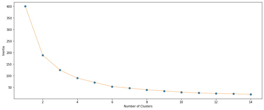
kmeans = KMeans(n_clusters=4)
kmeans.fit(X1)
cluster = kmeans.labels_
print(np.unique(cluster, return_counts=True)) #(array([0, 1, 2, 3]), array([38, 65, 47, 50], dtype=int64))

plt.figure(figsize=(15,7))
sns.scatterplot(x=X1[cluster==0, 0], y=X1[cluster==0, 1], color='yellow', label='Cluster 1', s=50)
sns.scatterplot(x=X1[cluster==1, 0], y=X1[cluster==1, 1], color='blue', label='Cluster 2', s=50)
sns.scatterplot(x=X1[cluster==2, 0], y=X1[cluster==2, 1], color='green', label='Cluster 3', s=50)
sns.scatterplot(x=X1[cluster==3, 0], y=X1[cluster==3, 1], color='grey', label='Cluster 4', s=50)
sns.scatterplot(x=kmeans.cluster_centers_[:, 0], y=kmeans.cluster_centers_[:,1], color='red'
                , label='Centroids', s=300, marker=',')
plt.grid(False)
plt.title('cluster of customers')
plt.xlabel('Age')
plt.ylabel('Spending Score (1-100)')
plt.legend()
plt.show()
new_df = df.copy()
new_df['label'] = cluster

from sklearn.metrics import silhouette_samples, silhouette_score
s_coefs = silhouette_samples(X1, cluster)
s_mean = silhouette_score(X1, cluster)
print(s_mean) #0.4383860846531993

new_df['silhouette'] = s_coefs
print(new_df.groupby('label')['silhouette'].mean())
# label
# 0    0.391685
# 1    0.541934
# 2    0.482486
# 3    0.297813
# Name: silhouette, dtype: float64

kmeans = KMeans(n_clusters=5)
kmeans.fit(X1)
cluster = kmeans.labels_
print(np.unique(cluster, return_counts=True)) (array([0, 1, 2, 3, 4]), array([42, 25, 57, 47, 29], dtype=int64))

plt.figure(figsize=(15,7))
sns.scatterplot(x=X1[cluster==0, 0], y=X1[cluster==0, 1], color='yellow', label='Cluster 1', s=50)
sns.scatterplot(x=X1[cluster==1, 0], y=X1[cluster==1, 1], color='blue', label='Cluster 2', s=50)
sns.scatterplot(x=X1[cluster==2, 0], y=X1[cluster==2, 1], color='green', label='Cluster 3', s=50)
sns.scatterplot(x=X1[cluster==3, 0], y=X1[cluster==3, 1], color='grey', label='Cluster 4', s=50)
sns.scatterplot(x=X1[cluster==4, 0], y=X1[cluster==4, 1], color='brown', label='Cluster 5', s=50)
sns.scatterplot(x=kmeans.cluster_centers_[:, 0], y=kmeans.cluster_centers_[:,1], color='red'
                , label='Centroids', s=300, marker=',')
plt.grid(False)
plt.title('cluster of customers')
plt.xlabel('Age')
plt.ylabel('Spending Score (1-100)')
plt.legend()
plt.show()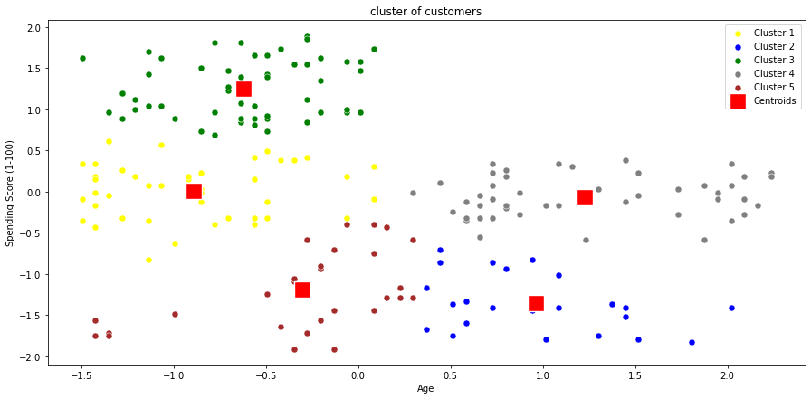
from yellowbrick.cluster
- KElbowVisualizer 함수 : 최적의 군집 수를 선택을 위한 Elbow method 구현
- SilhouetteVisualizer 함수 : 최적의 군집 수를 선택을 위한 Silhouette method 구현
from yellowbrick.cluster import KElbowVisualizer
df = pd.read_csv('../datas/Mall_Customers.csv')
X = df.iloc[:, 2:].values
model = KMeans(random_state=1)
visualizer = KElbowVisualizer(model, k=(2,10))
visualizer.fit(X)
visualizer.show()
plt.show()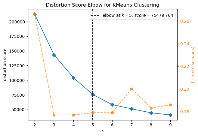
from yellowbrick.cluster import SilhouetteVisualizer
model = KMeans(n_clusters=5, random_state=1)
visualizer = SilhouetteVisualizer(model, metric='yellowbrick')
visualizer.fit(X)
visualizer.show()
plt.show()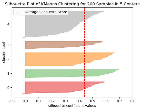
from sklearn.cluster import MiniBatchKMeans(속도향상)
class sklearn.cluster.MiniBatchKMeans(n_clusters=8, *, init='k-means++', max_iter=100, batch_size=1024, verbose=0, compute_labels=True, random_state=None, tol=0.0, max_no_improvement=10, init_size=None, n_init='warn', reassignment_ratio=0.01)
- batch size의 샘플들만 사용해서 중심점 update
- 성능 조금 희생 == inertia값, K-means보다 안 좋음
- 시간 대폭 줄여줌 == KMeans보다 3~4배 빠름
- batch_size 매개변수 : 각 배치에 랜덤하게 선택할 샘플의 수 조절
- partial_fit() : 데이터를 조금씩 전달하면서 훈련
- 참고 : https://box-world.tistory.com/62
from sklearn.cluster import MeanShift(평균이동)
- 클러스터 수나 모양을 가정하지 않고 샘플을 그룹으로 나눌 때 사용
- 참고 : https://romg2.github.io/mlguide/[Python] 머신러닝 완벽가이드 - 07. 군집화[평균 이동]
K-medoids
- K-means 변형 > 중간점(medoids) 사용
- 이상값에 좋은 성능 보임
- 데이터 간의 모든 거리 비용을 반복하여 계산 > 상대적으로 많은 시간 소요
- 최적의 K : Elbow method, Silhouette method
- 단점 : 원형x이면, 군집화 어려움
- 참고 : https://glorymind.tistory.com/entry/Kmedoids-Clustering-Algorithm
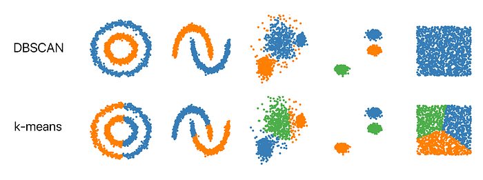
2. DBSCAN
(Density-based Spatial Clustering of Applications with Noise)
- 노이즈가 있는 대규모 데이터에 적용할 수 있는 밀도 기반 군집화 알고리즘
- 비선형 경계 클러스터링(불특정한 분포, 기하학적 모양의 군집도 잘 찾음)
- 연결되어 있는 데이터를 묶고 싶을 때 유용
- 저밀도 클러스터에서 고밀도 클러스터 분리에 유용
- 해당 알고리즘을 시행할 때마다 다른 결과 도출가능(데이터 포인트 처리 순서 매번 다름)
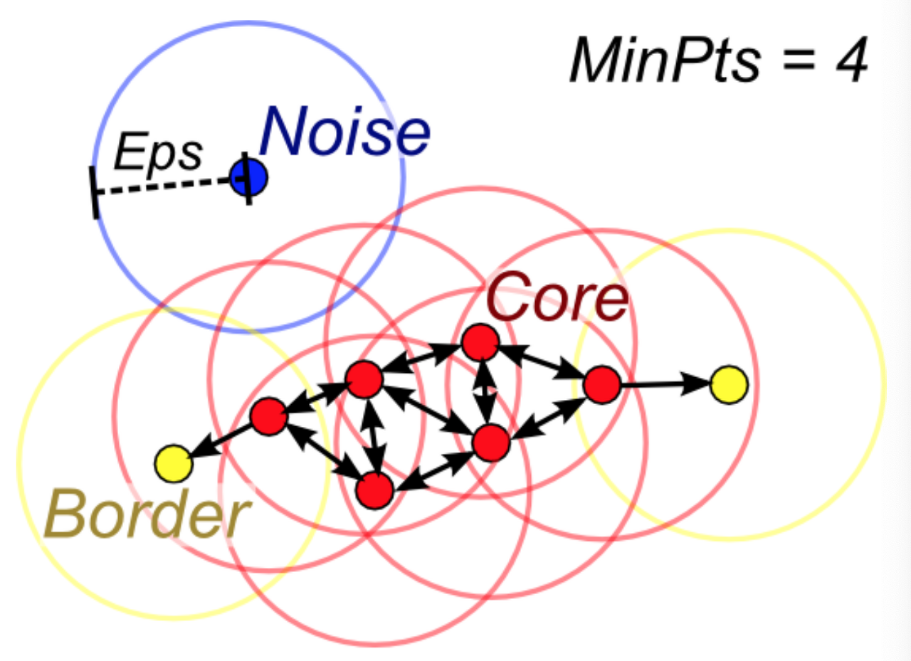
- 데이터세트의 각 요소 : 핵심(core) >> 경계(border) >> 이상치 요소(outlier point)
- eps와 minpts 결정해야 함
> 반경의 크기(=eps)
> 최소 군집의 크기(=MinPts) : 몇개가 연결되어 있어야 군집으로 볼 것인지의 개수
=> k-distance를 통해 적절한 값 결정(포인트 ~ k개의 가장 가까운 다른 데이터 평균거리) - R(Radius of neighborhood) : 특정 요소를 기준으로 반경 결정 = 밀도 영역(dense area)
- M(Min number of neighbors) : 핵심 요소 주변으로 요소가 몇개 있는지 지정
작동 순서
- 무작위 point 선택
- 선택된 point 에 대해 eps 거리 안의 모든 포인트 탐색
> 거리 안의 point 수 < min_samples : noise
> 거리 안의 point 수 > min_samples : core point, 새로운 클러스터 레이블 할당 - 할당된 point의 모든 이웃 확인
> 할당x : 직전에 만든 클러스터에 할당
> core point : core의 이웃 확인 - eps 거리 안에 더 이상 core point가 없을 때까지 3번 반복 > 방문 못한 데이터에 대해서 1번부터 반복
from sklearn.cluster import DBSCAN
class sklearn.cluster.DBSCAN(eps=0.5, *, min_samples=5, metric='euclidean', metric_params=None, algorithm='auto', leaf_size=30, p=None, n_jobs=None)
- eps : 다른 샘플을 이웃으로 고려하기 위한 최대 거리 (핵심 포인트를 중심으로 측정되는 유클리디언 거리값)
- min_samples : 핵심 샘플로 간주하기 위해 eps 거리 내에 필요한 최소 샘플 개수(기본 = 변수의개수 +1)
- metric : eps에서 사용할 거리 측정 방식
- core_sample_indices_속성 : 찾은 핵심 샘플의 인덱스
- fit_predict() : 예측 결과 확인
클러스터링 평가
1. Dunn Index
- 클수록 잘 분류됨
- 클러스터 간 최소 거리
_________________
클러스터 내 최대 거리 - 참고 : https://zephyrus1111.tistory.com/180
2. Silhouette Index
- 위의 실루엣 계수와 동일
- 클수록 잘 분류됨
- (클러스터들간의 평균 거리 최소값 - 동일한 클러스터내 데이터들의 평균거리)
_____________________________________________________________
max(클러스터들간의 평균 거리 최소값, 동일한 클러스터내 데이터들의 평균거리)
군집 알고리즘의 결과를 실제 정답 클러스터와 비교하여 평가할 수 있는 지표
1 : 최적 클러스터를 의미
0 : 무작위 클러스터를 의미
1. ARI (adjusted rand index)
- 수식참고 : https://taeguu.tistory.com/53
- sklearn.metrics.adjusted_rand_score(labels_true, labels_pred)
2. NMI (normalized mutual information)
- 수식참고 : https://process-mining.tistory.com/141
- sklearn.metrics.normalized_mutual_info_score(labels_true, labels_pred, *, average_method='arithmetic')
from sklearn import datasets
from sklearn.preprocessing import StandardScaler
from sklearn.cluster import KMeans, AgglomerativeClustering, DBSCAN
from sklearn.metrics.cluster import adjusted_rand_score, silhouette_score

X, y = datasets.make_moons(n_samples=200, noise=0.05, random_state=0)

kmeans = KMeans(n_clusters=2)
kmeans.fit(X)
y_pred = kmeans.predict(X)
plt.scatter(X[:, 0], X[:,1], c=y_pred, cmap=mglearn.cm2, s=60, edgecolors='k')
plt.scatter(kmeans.cluster_centers_[:,0], kmeans.cluster_centers_[:1], marker='^'
            , c=[mglearn.cm2(0), mglearn.cm2(1)], s=100, linewidths=2, edgecolors='k')
plt.xlabel('feature 0')
plt.ylabel('feature 1')
plt.show()
#실제 정답과 비교(ARI)
scaler = StandardScaler()
scaler.fit(X)
X_scale = scaler.transform(X)

random_state = np.random.RandomState(seed=0)
random_clusters = random_state.randint(low=0, high=2, size=len(X))
fig, axes = plt.subplots(1,4, figsize=(15,3), subplot_kw={'xticks':(), 'yticks':()})
algorithms = [KMeans(n_clusters=2), AgglomerativeClustering(n_clusters=2), DBSCAN()]

#무작위 할당 클러스터 그림
axes[0].scatter(X_scale[:, 0], X_scale[:,1], c=random_clusters, cmap=mglearn.cm3, s=60, edgecolors='black')
axes[0].set_title("Randomly - ARI : {:.2f}".format(adjusted_rand_score(y, random_clusters)))

for ax, algorithm in zip(axes[1:], algorithms):
    # 클러스터 할당과 클스터 중심을 그림
    clusters = algorithm.fit_predict(X_scale)
    ax.scatter(X_scale[:, 0], X_scale[:, 1], c=clusters,
               cmap=mglearn.cm3, s=60, edgecolors='black')
    ax.set_title("{} - ARI: {:.2f}".format(algorithms.__class__.__name__, adjusted_rand_score(y,clusters)))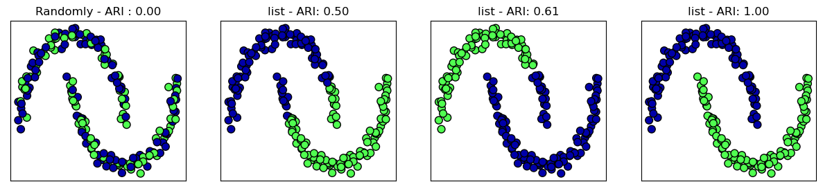
#실제 정답과 비교(silhouette index)
fig, axes = plt.subplots(1,4, figsize=(15,3), subplot_kw={'xticks':(), 'yticks':()})
algorithms = [KMeans(n_clusters=2), AgglomerativeClustering(n_clusters=2), DBSCAN()]

#무작위 할당 클러스터 그림
axes[0].scatter(X_scale[:, 0], X_scale[:,1], c=random_clusters, cmap=mglearn.cm3, s=60, edgecolors='black')
axes[0].set_title("Randomly - silhouette : {:.2f}".format(silhouette_score(X_scale, random_clusters)))

for ax, algorithm in zip(axes[1:], algorithms):
    # 클러스터 할당과 클스터 중심을 그림
    clusters = algorithm.fit_predict(X_scale)
    ax.scatter(X_scale[:, 0], X_scale[:, 1], c=clusters,
               cmap=mglearn.cm3, s=60, edgecolors='black')
    ax.set_title("{} - silhouette: {:.2f}".format(algorithms.__class__.__name__, silhouette_score(X_scale,clusters)))
* 내용참고&출처 : 태그의 수업을 복습 목적으로 정리한 내용입니다.
'IT > ML' 카테고리의 다른 글
| [sklearn] 사이킷런 (scikit-learn) 주요 모듈 (0) | 2022.11.20 |
|---|---|
| [Machine Learning] 오차행렬 - 모델 평가&분류 확인 (0) | 2022.11.20 |
| [Machine Learning] 군집분석; Hierarchical clustering (0) | 2022.11.17 |
| [Machine Learning] Sampling (0) | 2022.11.11 |
| [sklearn] kNN(k-Nearest Neighbors) (0) | 2022.11.11 |

